|
Multidimensional Scaling
Overview
From a non-technical point of view, the purpose of multidimensional scaling (MDS) is to provide a visual representation of the pattern of proximities (i.e., similarities or distances) among a set of objects. For example, given a matrix of perceived similarities between various brands of air fresheners, MDS plots the brands on a map such that those brands that are perceived to be very similar to each other are placed near each other on the map, and those brands that are perceived to be very different from each other are placed far away from each other on the map.

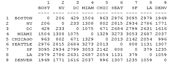
For instance, given the matrix of distances among cities shown
above, MDS produces this map:
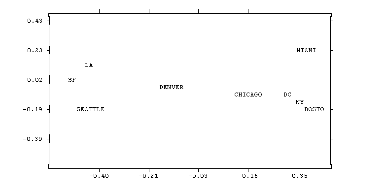
In this example, the relationship between input proximities
and distances among points on the map is positive: the smaller
the input proximity, the closer (smaller) the distance between
points, and vice versa. Had the input data been similarities, the
relationship would have been negative: the smaller the input
similarity between items, the farther apart in the picture they
would be.
From a slightly more technical point of view, what MDS does is
find a set of vectors in p-dimensional space such that the matrix
of euclidean distances among them corresponds as closely as
possible to some function of the input matrix according to a
criterion function called stress.
A simplified view of the algorithm is as follows:
Input Data
The input to MDS is a square, symmetric 1-mode matrix
indicating relationships among a set of items. By convention,
such matrices are categorized as either similarities or
dissimilarities, which are opposite poles of the same continuum.
A matrix is a similarity matrix if larger numbers indicate more
similarity between items, rather than less. A matrix is a
dissimilarity matrix if larger numbers indicate less
similarity. The distinction is somewhat misleading, however,
because similarity is not the only relationship among items that
can be measured and analyzed using MDS. Hence, many input
matrices are neither similarities nor dissimilarities.
However, the distinction is still used as a means of
indicating whether larger numbers in the input data should mean
that a given pair of items should be placed near each other on
the map, or far apart. Calling the data "similarities"
indicates a negative or descending relationship between input
values and corresponding map distances, while calling the data
"dissimilarities" or "distances" indicates a
positive or ascending relationship.
A typical example of an input matrix is the aggregate
proximity matrix derived from a pilesort task. Each cell xij
of such a matrix records the number (or proportion) of
respondents who placed items i and j into the
same pile. It is assumed that the number of respondents placing
two items into the same pile is an indicator of the degree to
which they are similar. An MDS map of such data would put items
close together which were often sorted into the same piles.
Another typical example of an input matrix is a matrix of
correlations among variables. Treating these data as similarities
(as one normally would), would cause the MDS program to put
variables with high positive correlations near each other, and
variables with strong negative correlations far apart.
Another type of input matrix is a flow matrix. For example, a
dataset might consist of the number of business transactions
occurring during a given period between a set of corporations.
Running this data through MDS might reveal clusters of
corporations that whose members trade more heavily with one
another than other than with outsiders. Although technically
neither similarities nor dissimilarities, these data should be
classified as similarities in order to have companies who trade
heavily with each other show up close to each other on the map.
Dimensionality
Normally, MDS is used to provide a visual representation of a
complex set of relationships that can be scanned at a glance.
Since maps on paper are two-dimensional objects, this translates
technically to finding an optimal configuration of points in
2-dimensional space. However, the best possible configuration in
two dimensions may be a very poor, highly distorted,
representation of your data. If so, this will be reflected in a
high stress value. When this happens, you have two choices: you
can either abandon MDS as a method of representing your data, or
you can increase the number of dimensions.
There are two difficulties with increasing the number of
dimensions. The first is that even 3 dimensions are difficult to
display on paper and are significantly more difficult to
comprehend. Four or more dimensions render MDS virtually useless
as a method of making complex data more accessible to the human
mind.
The second problem is that with increasing dimensions, you
must estimate an increasing number of parameters to obtain a
decreasing improvement in stress. The result is model of the data
that is nearly as complex as the data itself.
On the other hand, there are some applications of MDS for
which high dimensionality is not a problem. For instance, MDS can
be viewed as a mathematical operation that converts an
item-by-item matrix into an item-by-variable matrix. Suppose, for
example, that you have a person-by-person matrix of similarities
in attitudes. You would like to explain the pattern of
similarities in terms of simple personal characteristics such as
age, sex, income and education. The trouble is, these two kinds
of data are not conformable. The person-by-person matrix in
particular is not the sort of data you can use in a regression to
predict age (or vice-versa). However, if you run the data through
MDS (using very high dimensionality in order to achieve perfect
stress), you can create a person-by-dimension matrix which is
similar to the person-by-demographics matrix that you are trying
to compare it to.
Stress
The degree of correspondence between the distances among
points implied by MDS map and the matrix input by the user is
measured (inversely) by a stress function. The general
form of these functions is as follows:

In the equation, dij refers to
the euclidean distance, across all dimensions, between points i
and j on the map, f(xij)
is some function of the input data, and scale refers to
a constant scaling factor, used to keep stress values between 0
and 1. When the MDS map perfectly reproduces the input data, f(xij)
- dij is for all i and j,
so stress is zero. Thus, the smaller the stress, the better the
representation.
The stress function used in ANTHROPAC is variously called "Kruskal Stress", "Stress Formula 1" or just "Stress 1". The formula is:

The transformation of the input values f(xij)
used depends on whether metric or non-metric scaling. In metric
scaling, f(xij) = xij.
In other words, the raw input data is compared directly to the
map distances (at least in the case of dissimilarities: see the
section of metric scaling for information on similarities). In
non-metric scaling, f(xij)
is a weakly monotonic transformation of the input data that
minimizes the stress function. The monotonic transformation is
computed via "monotonic regression", also known as
"isotonic regression".
From a mathematical standpoint, non-zero stress values occur
for only one reason: insufficient dimensionality. That is, for
any given dataset, it may be impossible to perfectly represent
the input data in two or other small number of dimensions. On the
other hand, any dataset can be perfectly represented using n-1
dimensions, where n is the number of items scaled. As
the number of dimensions used goes up, the stress must either
come down or stay the same. It can never go up.
Of course, it is not necessary that an MDS map have zero
stress in order to be useful. A certain amount of distortion is
tolerable. Different people have different standards regarding
the amount of stress to tolerate. The rule of thumb we use is
that anything under 0.1 is excellent and anything over 0.15 is
unacceptable. Care must be exercised in interpreting any map that
has non-zero stress since, by definition, non-zero stress means
that some or all of the distances in the map are, to some degree,
distortions of the input data. The distortions may be spread out
over all pairwise relationships, or concentrated in just a few
egregious pairs. In general, however, longer distances tend to be
more accurate than shorter distances, so larger patterns are
still visible even when stress is high. See the section on
Shepard Diagrams and Interpretation for further information on
this issue.
From a substantive standpoint, stress may be caused either by
insufficient dimensionality, or by random measurement error. For
example, a dataset consisting of distances between buildings in
New York City, measured from the center of the roof, is clearly
3-dimensional. Hence we expect a 3-dimensional MDS configuration
to have zero stress. In practice, however, there is measurement
error such that a 3-dimensional solution does not have zero
stress. In fact, it may be necessary to use 8 or 9 dimensions to
bring stress down to zero. In this case, the fact that the
"true" number of dimensions is known to be three allows
us to use the stress of the 3-dimensional solution as a direct
measure of measurement error. Unfortunately, in most datasets, it
is not known in advance how many dimensions there
"really" are.
In such cases we hope (with little foundation) that the true
dimensionality of the data will be revealed to us by the rate of
decline of stress as dimensionality increases. For example, in
the distances between buildings example, we would expect
significant reductions in stress as we move from a one to two to
three dimensions, but then we expect the rate of change to slow
as we continue to four, five and higher dimensions. This is
because we believe that all further variation in the data beyond
that accounted for by three dimensions is non-systematic noise
which must be captured by a host of "specialized"
dimensions each accounting for a tiny reduction in stress. Thus,
if we plot stress by dimension, we expect the following sort of
curve:
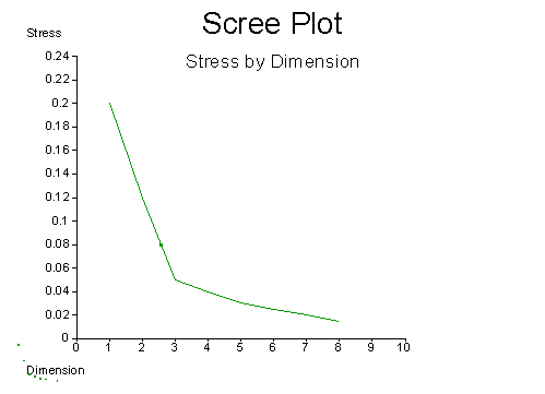
Thus, we can theoretically use the "elbow" in the
curve as a guide to the dimensionality of the data. In practice,
however, such elbows are rarely obvious, and other, theoretical,
criteria must be used to determine dimensionality.
Shepard Diagrams
The Shepard diagram is a scatterplot of input proximities
(both xij and f(xij))
against output distances for every pair of items scaled.
Normally, the X-axis corresponds to the input proximities and the
Y-axis corresponds to both the MDS distances dij
and the transformed ("fitted") input proximities f(xij).
An example is given in Figure 3. In the plot, asterisks mark
values of dij and dashes mark values
of f(xij). Stress measures
the vertical discrepancy between xij
(the map distances) and f(xij)
(the transformed data points). When the stress is zero, the
asterisks and dashes lie on top of each other. In metric scaling,
the asterisks form a straight line. In nonmetric scaling, the
asterisks form a weakly monotonic function(1),
the shape of which can sometimes be revealing (e.g., when
map-distances are an exponential function of input proximities).
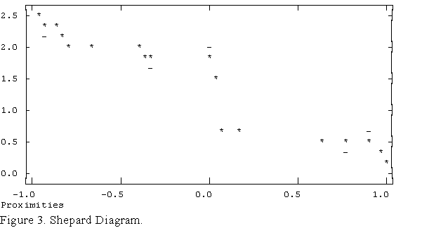
If the input proximities are similarities, the points should
form a loose line from top left to bottom right, as shown in
Figure 3. If the proximities are dissimilarities, then the data
should form a line from bottom left to top right. In the case of
non-metric scaling, f(xij)
is also plotted.
At present, the ANTHROPAC program does not print Shepard
diagrams. It does, however, print out a list of the most
discrepant (poorly fit) pairs of items. If you notice that the
same item tends to appear in a number of discrepant pairs, it
would make sense to delete the item and rerun the scaling.
Interpretation
There are two important things to realize about an MDS map.
The first is that the axes are, in themselves, meaningless and
the second is that the orientation of the picture is arbitrary.
Thus an MDS representation of distances between US cities need
not be oriented such that north is up and east is right. In fact,
north might be diagonally down to the left and east diagonally up
to the left. All that matters in an MDS map is which point is
close to which others.
When looking at a map that has non-zero stress, you must keep
in mind that the distances among items are imperfect, distorted,
representations of the relationships given by your data. The
greater the stress, the greater the distortion. In general,
however, you can rely on the larger distances as being accurate.
This is because the stress function accentuates discrepancies in
the larger distances, and the MDS program therefore tries harder
to get these right.
There are two things to look for in interpreting an MDS
picture: clusters and dimensions. Clusters are groups of items
that are closer to each other than to other items. For example,
in an MDS map of perceived similarities among animals, it is
typical to find (among north americans) that the barnyard animals
such as chicken, cow, horse, and pig are all very near each
other, forming a cluster. Similarly, the zoo animals like lion,
tiger, antelope, monkey, elephant and giraffe form a cluster.
When really tight, highly separated clusters occur in perceptual
data, it may suggest that each cluster is a domain or subdomain
which should be analyzed individually. It is especially important
to realize that any relationships observed within such a cluster,
such as item a being slightly closer to item b
than to c should not be trusted because the exact
placement of items within a tight cluster has little effect on
overall stress and so may be quite arbitrary. Consequently, it
makes sense to extract the submatrix corresponding to a given
cluster and re-run the MDS on the submatrix.(2)
(In some cases, however, you will want to re-run the data
collection instead.)
Dimensions are item attributes that seem to order the items in
the map along a continuum. For example, an MDS of perceived
similarities among breeds of dogs may show a distinct ordering of
dogs by size. The ordering might go from right to left, top to
bottom, or move diagonally at any angle across the map. At the
same time, an independent ordering of dogs according to
viciousness might be observed. This ordering might be
perpendicular to the size dimension, or it might cut a sharper
angle.
The underlying dimensions are thought to "explain"
the perceived similarity between items. For example, in the case
of similarities among dogs we expect that the reason why two dogs
are seen as similar is because they have locations or scores on
the identified dimensions. Hence, the observed similarity between
a doberman and a german shepherd is explained by the fact that
they are seen as nearly equally vicious and about the same size.
Thus, the implicit model of how similarity judgments are produced
by the brain is that items have attributes (such as size,
viciousness, intelligence, furriness, etc) in varying degrees,
and the similarity between items is a function of their
similarity in scores across all attributes. This function is
often conceived of as a weighted sum of the similarity across
each attribute, where the weights reflect the importance or
saliency of the attribute.
It is important to realize that these substantive dimensions
or attributes need not correspond in number or direction to the
mathematical dimensions (axes) that define the vector space (MDS
map). For example, the number of dimensions used by respondents
to generate similarities may be much larger than the number of
mathematical dimensions needed to reproduce the observed pattern.
This is because the mathematical dimensions are necessarily
orthogonal (perpendicular), and therefore maximally efficient. In
contrast, the human dimensions, while cognitively distinct, may
be highly intercorrelated and therefore contain some redundant
information.
One thing to keep in mind in looking for dimensions is that
your respondents may not have the same views that you do. For one
thing, they may be reacting to attributes you have not thought
of. For another, even when you are both using the same set of
attributes, they may assign different scores on each attribute
than you do. For example, one of the attributes might be
"attractiveness". Your view of what an attractive dog,
person, fruit or other item may be very different from your
respondents'.(3)
Useful References
Methodological
Applications
1. If the input data dissimilarities, the function is never decreasing. If the input data are similarities, the function is never increasing.
2. In some cases, however, it is better to rerun the data collection on the subset of items. This is because the presence of the other items can evoke additional dimensions/attributes of comparison that could affect the way items in the subset are viewed.
3. Fortunately, a very simple technique exists to deal with this problem. The technique is called property fitting (PROFIT).
[geneva97/eop.htm]