|
Proximities
Overview
A proximity is a measurement of the similarity or
dissimilarity, broadly defined, of a pair of objects. If measured
for all pairs of objects in a set (e.g. driving distances among a
set of U.S. cities), the proximities are represented by an
object-by-object proximity matrix, such as the following distance
matrix:

A proximity is thought of as a similarity if the
larger the value for a pair of objects, the closer or more alike
we think they are. Examples of similarities are co-occurrences,
interactions, statistical correlations and associations, social
relations, and reciprocals of distances. A proximity is a dissimilarity
if the smaller the value for a pair of objects, the closer
or more alike we think of them. Examples are distances,
differences, and reciprocals of similarities.
Proximities are normally symmetric, so that the proximity of
object a to object b is the same as the
proximity of object b to object a. For example,
the distance from Boston to NY is 206 miles, and the distance
from NY to Boston is also 206 miles. However, in the case of
one-way streets, it is possible for distances to be
non-symmetric.
There are two basic ways of obtaining proximity: directly (or dyadically)
and indirectly (or monadically). Direct measures are
obtained in the obvious way. For example, a direct measure of
distance between cities is obtained by driving from one city to
the other. A direct measure of interaction between two people is
obtained by counting the number of times that they speak to each
other over a given period.
Indirect measures are obtained by first measuring the objects
on one or more attributes. This is recorded as a 2-way, 2-mode
object-by-attribute matrix. The set of scores associated with an
object or an attribute (that is, a row or a column of the data
matrix) is called a profile. Then, a statistical measure
of the similarity or dissimilarity of profiles is computed for
each pair of objects or attributes (i.e., each pair of rows or
columns of the data matrix).
In many situations, the objects are thought of as cases
and the attributes are seen as variables.

Hundreds of measures are available. The choice of measure is
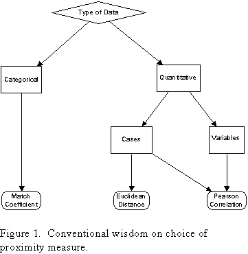
determined in part by the type of data (see Figure 1). For
categorical data, the typical measure is the match
coefficient, which, for a given pair of objects, is simply
the count of the number of times (attributes/columns) that one
object has the exact same value as the other object. Typically,
this count is then divided by the maximum possible, which is
normally the total number of attributes/columns in the data (that
both objects have non-missing values for). For example, if the
people are objects
For quantitative data, two measures are commonly used, one a
similarity measure (correlation) and the other a dissimilarity
measure (euclidean distance). Typically, Euclidean distance is
only used to measure proximities among cases (generally
respondents), whereas correlation tends to be used to measure
proximities among variables (generally attributes of the
respondents).
The key issue in choosing a measure of proximity for
quantitative data is what aspects of profiles we would like to
the measure to attend to. Every profile can be said to possess
three aspects: level, amplitude (or scatter), and pattern. Level
refers to the general size of the numbers and is measured by the
mean of all the values. Amplitude refers to the extremeness or
variability of the numbers and is measured by the standard
deviation. Pattern refers to the sequence of ups and downs in the
values as we move from case to case. It is not measureable in
isolation. We can ask whether two profiles have the same pattern,
and even how different they are from each other, but there is no
monadic measurement of pattern.
The Euclidean distance between two profiles is a function of
differences in mean, differences in amplitude, and differences in
pattern, all take together. Only if two profiles are the same
across all three aspects will Euclidean distance say they are the
same. In contrast, correlation ignores differences in level and
amplitude, and pays attention only to differences in pattern. For
example, if we were to measure the income in dollars of a sample
of people, then change the units to thousands of dollars (so that
$15,500 becomes $15.5), the amplitude of the variable would be
reduced by a factor of 100, but the correlation between the two
versions of income would be a perfect 1.0.
The reason why Euclidean distance is typically not used for
comparing variables is that variables often have wildly different
units of measurement. If we compare respondents' income (in
dollars) with their education (in years), we will find a massive
Euclidean distance between the variables, even if their patterns
are identical (that is, when one variable is high relative to
other cases, the other variable is high relative to other cases,
and vice-versa).
So the only time we use Euclidean distances is when
differences in scale (i.e., level and amplitude) are meaningful.
For example, suppose our data consist of demographic information
on a sample of individuals, arranged as a respondent-by-variable
matrix. Each row of the matrix is a profile of m
numbers, where m is the number of variables. We can
evaluate the proximity (in this case, the distance) between any
pair of rows. Now, consider what it means, for a moment, that the
variables are the columns. A variable records the results of a
measurement. For our purposes, in fact, it is useful to think of
the variable as the measuring device itself. This means that it
has its own scale, which determines the size and type of numbers
it can have. For instance, the income measurer might yield
numbers between 0 and 79 million, while another variable, the
education measurer, might yield numbers from 0 to 30. The fact
that income numbers are larger in general than the education
numbers is not meaningful because the variables are measured on
different scales. In order to compare columns we must adjust for
or take account of differences in scale. But the row vectors are
different. If one case has larger numbers in general then another
case, this is because that case has more income, more education,
etc. than the other case; it is not an artifact of differences in
scale, because rows do not have scales: they are not even
variables. In order to compute similarities or dissimilarities
among rows, we do not need to (in fact, must not) try to adjust
for differences in scale. Hence, euclidean distance is usually
the right measure for comparing cases.
Euclidean Distance
Euclidean distance is defined as the square root of the sum of
squared differences between two profiles. For example, the
Euclidean distance between profiles A and B below is 30
(1+1+1+1+0+4+16+1+1+4).
| Object | Attributes (Profile) | |||||||||
| A | 3 | 5 | 3 | 2 | 5 | 4 | 1 | 5 | 1 | 4 |
| B | 4 | 4 | 2 | 3 | 5 | 2 | 5 | 4 | 2 | 2 |
| 12 | 12 | 12 | 12 | 02 | 22 | 42 | 12 | 12 | 22 | |
Note that Euclidean distance is not clearly bounded -- it runs
from zero (when the profiles are identical) to an unknown
maximum. Furthermore, it is sensitive to the scale of numbers
(the level and amplitude). If we were to add 10 to every value in
profile A, or multiply every value by 10, the Euclidean distance
between the profiles would increase.
Pearson Correlation
The correlation between profiles X and Y is defined as
follows:

where µX and µY are the means of X and
Y respectively, and X and Y are the
standard deviations of X and Y. The numerator of the equation is
called the covariance of X and Y, and is the difference between
the mean of the product of X and Y subtracted from the product of
the means. Note that if X and Y are standardized, they will each
have a mean of 0 and a standard deviation of 1, so the formula
reduces to:

Whereas euclidean distance was the sum of squared differences,
correlation is basically the average product. There is a further
relationship between the two. If we expand the formula for
euclidean distance, we get this:

But if X and Y are standardized, the sums x2 and y2
are both equal to n. That leaves xy as the only
non-constant term, just as it was in the reduced formula for the
correlation coefficient. Thus, for standardized data, we can
write the correlation between X* and Y* in
terms of the squared distance between them:

Hence, for standardized data (where level and amplitude
differences are removed), correlation is a simple linear
transformation of Euclidean distance squared.
Step-by-Step
1. Collect data for a person-by-method matrix which contains a
1 if a given person has used a given statistical method, and 0
otherwise. Here is a hypothetical example of such a matrix:
| Correlation | Regression | ANOVA | MDS | FACTOR | Chi-square | Log-Linear | |
| Bill | 1 | 1 | 1 | 0 | 1 | 0 | 0 |
| John | 1 | 0 | 0 | 1 | 1 | 0 | 0 |
| Mary | 0 | 0 | 1 | 0 | 0 | 1 | 1 |
| Don | 0 | 0 | 1 | 1 | 0 | 1 | 0 |
| Jan | 1 | 1 | 0 | 0 | 0 | 1 | 0 |
| Sally | 0 | 1 | 1 | 0 | 0 | 1 | 1 |
Note that these data could be treated as either
categorical or quantitative. Furthermore, although the rows
appear to be cases and the columns variables, the units of
measurement are the same across the board. Consequently, we can
use all three measures discussed above.
2. Enter the data into an ascii file called
STATMETH.DAT using the following format:

3. Import the data as a dataset called
STATMETH.
Proximities Among Persons
1. Choose TOOLS>SIMILARITIES from the menu.
Fill in the input form as shown below:

To run the program, press F10. The result
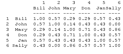
should be the following matrix:

As you can see, the similarity between Bill and
John is given as 0.57. This is because Bill and John give exactly
the same answer (whether "1" or "0" makes no
difference) on 4 out of 7 questions, which is 57% to two decimal
places.
2. Choose TOOLS>SIMILARITIES from the menu.
Fill in the input form as shown below (note change of measure to
CORRELATION):

To run the program, press F10. The result
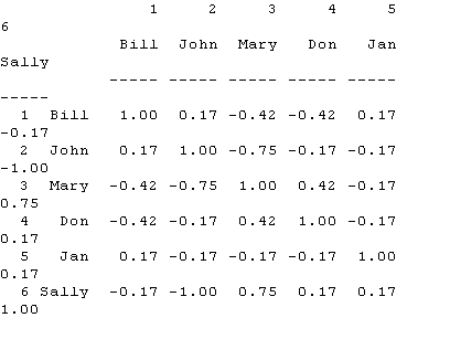
should be the following matrix:

Note that the numbers have changed, but the
pattern is fairly similar. Looking at Bill's correlations with
others we see they are highest with John and Jan, lowest (in
fact, negative) with Mary and Don, and in between with Sally. The
same is true in the similarity matrix obtained using the match
coefficient.
3. Choose TOOLS>DISSIMILARITIES from the
menu (note change to dissimilarities). Fill in the input form as
shown below.

To run the program, press F10. The result
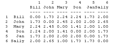
should be the following matrix:

Note that the numbers have not only changed but
reversed. Looking at Bill's proximities with others we see they
are lowest with John and Jan, highest with Mary and Don, and in
between with Sally. This is exactly the opposite of our previous
two results.
Proximities Among Methods
To compute proximities among each pair of
methods, just repeat the process above, but change
"ROWS" to "COLUMNS" in every case. The result
in each case will be a method-by-method proximity matrix. For
example, in the case of the matches coefficient, the matrix will
give the extent to which each pair of methods was used by exactly
the same individuals.
References
Methodological
Liebetrau. Measures of Association. Sage.
SPSS, Inc. "Proximities." SPSS
Reference Guide. Pp. 550-562.
Applications
Boster & Johnson 1989. "Form or function: A comparison of expert and novice judgements of similarity among fish." American Anthropologist 91:866-889.
Byrne & Forline 1993. "Brazilian emic
use of physical cues to ascribe social race identity" Unpublished
manuscript, University of Florida.