The Average and the Histogram

(From Statistics, by Freedman, Pisani, Purves, Adhikari).

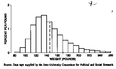
This section will indicate how the average and the median are related to histograms. To begin with an example, figure 4 shows a histogram for the weights of the 6,588 women age 18-74 in the HANES sample. The average (146 pounds) is marked with a vertical line. It is natural to guess that 50% of the women were above average in weight, and 50% were below average. However, this guess is somewhat off. In fact, only 41 % were above average; the remaining 59% were below average. And in other situations, the percentages can be even farther from 50%.

Figure 4. Histogram for the weights of the 6,588 women in the HANES sample. The average is marked by the dashed line. Only 41% of the women are above average in weight.

How is this possible? To find out, it is easiest to start with some hypothetical data-the list 1, 2, 2, 3. The histogram for this list (figure 5) is symmetric about the value 2. That is, imagine drawing a vertical line through the value 2, and folding the histogram in half around that line: the two halves would match up. And the average equals 2. If the histogram is symmetric around a value, that value equals the average; furthermore, half the area under the histogram lies to the left of that value, and half to the right.

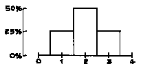Figure 5. Histogram for the list 1, 2, 2, 3. The histogram is symmetric around 2, the average; 50% of the area is to the left of 2, and 50% to the right.

What happens when the value 3 on the list 1, 2, 2, 3 is increased, say to 5 or 7? As shown in figure 6, the rectangle over that value moves off to the right, destroying the symmetry. The average for each histogram is marked with an arrow, and the arrow shifts to the right following the rectangle. To see why, imagine the histogram is made out of wooden blocks attached to a stiff, weight-less board. Put the histogram across a taut wire, as illustrated in the bottom panel of figure 6. The histogram will balance at the average. A small area far away from the average can balance a large area close to the average, because areas are weighted by their distance from the balance point.

NOTE: A histogram balances when supported at the average.

It is just like a seesaw: a small child sits farther away from the center in order to balance a large child sitting closer to the center. And that is why the percentage of cases on either side of the average can differ from 50%.

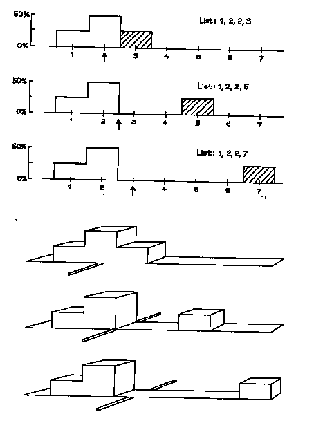Figure 6. The average. The top panel shows three histograms; the averages are marked by arrows. As the shaded box moves to the right, it pulls the average along with it. The area to the left of the average gets up to 75%. The bottom panel shows the same three histograms made out of wooden blocks attached to a stiff, weightless board. The histograms balance when supported at the average.

The median of a histogram is the value with half the area to the left and half to the right. In the third histogram of figure 6, the median is 2. The area to the right of the median is far away by comparison with the area to the left. Consequently, if you tried to balance this histogram at the median, it would tip to the right. More generally, the average is to the right of the median whenever the histogram has a long right-hand tail, as illustrated in figure 7. The weight histogram (figure 4 on p. 57) had a long right-hand tail; that is why the average was bigger than the median.

Figure 7. The tails of a histogram.

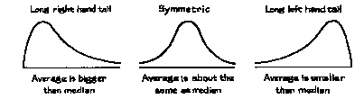
For another example, median family income in the United States in 1987 was about $30,800. The income histogram has a long right-hand tail, and the average was higher-$37'000. Statisticians often use the median rather than the average when dealing with long-tailed distributions, the reason being that in some cases the average pays too much attention to a small percentage of cases in the extreme tail of the distribution.

Technical note. The median of a list is defined so that half or more of the entries are at the median or bigger, and half or more are at the median or smaller. This will be illustrated on 4 lists:

(a) 1, 5, 7

(b) 1, 2, 5, 7

(c) 1, 2, 2, 7, 8

(d) 8, - 3, 5, 0, 1, 4, - I

For list (a), the median is 5: two entries out of the three are 5 or more, and two are 5 or less. For list (b), any value between 2 and 5 is a median; if pressed, most statisticians would choose 3.5 (which is halfway between 2 and 5) as "the" median. For list (c), the median is 2: four entries out of five are 2 or more, and three are 2 or less. To find the median of list (d), arrange it in increasing order:

-3, - 1, 0, 1, 4, 5, 8

There are seven entries on this list: four are 1 or more, and four are 1 or less. So 1 is the median.