The Regression Line

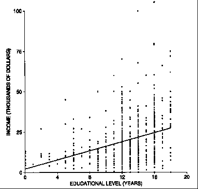
Does education pay? Figure 1 shows the relationship between income and education, for a representative sample of 637 California men age 25-29 in 1988. The summary statistics are:

average education is 12.5 years, SD is 4 years
average income is $19,700, SD is $16,000,
r = 0.35

The regression estimates for average income at each educational level fall along the regression line shown in the figure. The line slopes up, showing that on the average, income does go up with education.

Figure 1. The regression line. The scatter diagram shows
income and education for a representative sample of 637
California men age 25-29 in 1988.

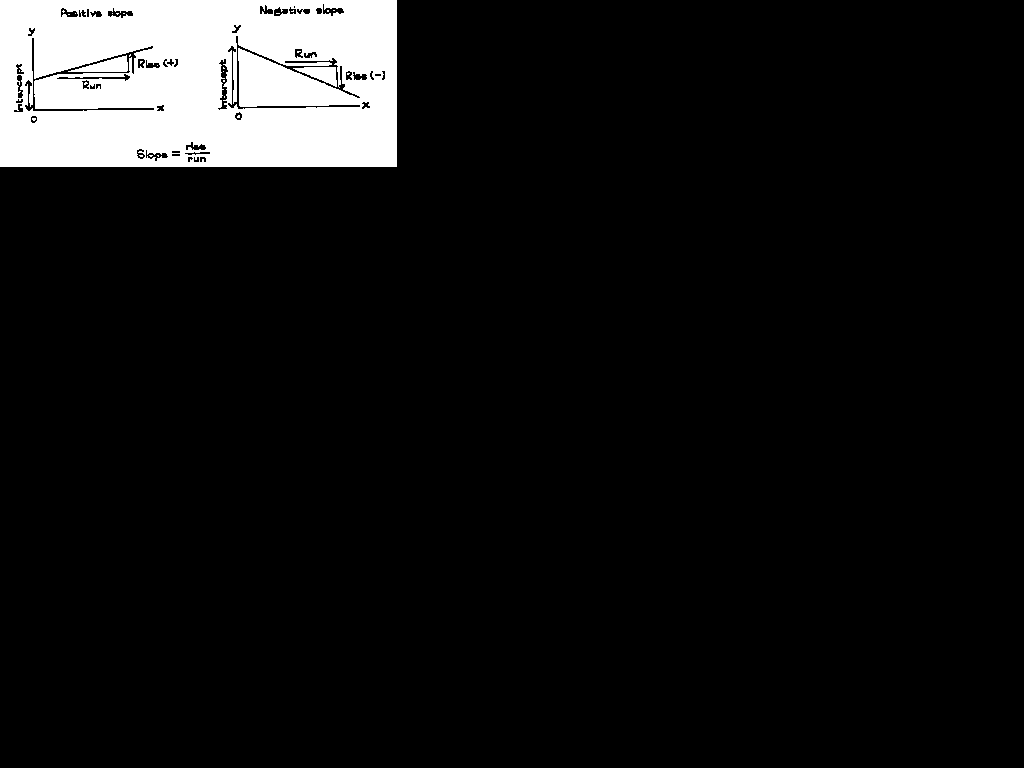
Any line can be described in terms of its slope and intercept. The y-intercept is the height of the line when x is 0. And the slope is the rate at which y increases, per unit increase in x. Slope and intercept are illustrated in figure 2.

Figure 2. Slope and intercept.

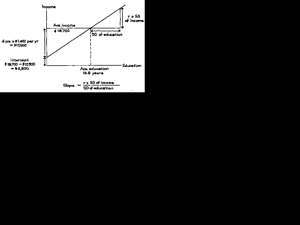
What do the slope and intercept mean for the regression line? To continue with the income-education example: associated with an increase of one SD in education, there is an increase of r SDs in income. That is, 4 extra years of education are worth an extra 0.35 x $16,000 = $5,600 of income, on the average. So each extra year is worth $5,600/4 = $1,400. The slope of the regression line is $1,400 per year. So far, it looks like education does pay off for the men, at the rate of $1,400 per year.

Figure 3. Finding the slope and intercept of the regression line.

The intercept of the regression line is its height when x = 0, corresponding to men with 0 years of education. Such men are 12.5 years below average in education. And each year costs $1,400-that is what the slope says. A man with no education is predicted to have an income which is below average by

12.5 years x $1,400 per year = $17,500.

So, his income is predicted as $19,700 - $17,500 = $2,200. This is the intercept: the predicted value of y when x = 0. (See figure 3.)

Zero years of education may sound extreme, but there were several men who reported having no education, and their incomes ranged from $0 to about $12,000; their points are in the lower left corner of figure 1.

Any line has an equation, in terms of its slope and intercept:

y = slope x x + intercept.

The equation for the regression line is called (not surprisingly) the regression equation. In Figure 3, the regression equation is

predicted income = ($1,400 per year) x education + $2,200.

There is nothing new here: the regression equation is just an alternative way of using the regression method to predict y from x. However, the regression equation is often used in the social sciences. An investigator who has to make many predictions might find it easier to compute the slope and intercept once and for all, and then substitute into the equation. Furthermore, the slope and intercept can be interesting in their own right.

Example 1. For 676 California women age 25-29 in 1988, there is a relationship between income and education; data are from the Current Population Survey. The relationship can be summarized as follows.

average education 12 years, SD 3.5 years
average income $11,600, SD $10,500,
r = 0.4

(a) Find the regression equation for predicting income from education.

(b) Use the equation to predict the income of a woman whose educational level is: 8 years, 12 years, 16 years.

Solution. Part (a). The first step is to find the slope (figure 3). In a run of one SD of education, the regression line rises r SDs of income. So

slope = (0.4 x $10,500)/3.5 years = $1,200 per year.

The interpretation: on the average, each extra year of schooling is worth an extra $1,200 of income; each year less of schooling costs $1,200 of income.

The next step is to find the intercept. That is the height of the regression line at x = 0. In other words, it is the predicted income of a woman with no education. Such a woman is 12 years below average; using the slope, she is predicted to be below average in income by

12 years x $1,200 per year = $14,400.

So her income is predicted as

$11,600 - $14,400 = -$2,800.

That is the intercept: the prediction for y when x = 0. (The regression line becomes less and less reliable as you move away from the center of the data, so a negative intercept is not too disturbing.) The regression equation is

predicted income = ($1,200 per year) x (education) - $2,800.

Part (b). Substituting 8 years for education gives

($1,200 per year) x (8 years) - $2,800 = $6,800.

Substituting 12 years for education gives

($1,200 per year) x (12 years) - $2,800 = $11,600.

Substituting 16 years for education gives

($1,200 per year) x (16 years) - $2,800 = $16,400.

This completes the solution. Despite the negative intercept, the predictions are quite reasonable -- for most of the women.

In this example, the slope is $1,200 per year. Associated with each extra year of education, there is an increase of $1,200 in income, on the average. The phrase "associated with" sounds like it is talking around some difficulty, and here is the issue: Are income differences caused by differences in educational level, or do both reflect the common influence of some third variable? The phrase "associated with" was invented to let statisticians talk about regressions without having to commit themselves on this sort of point.

Often, the slope is used to predict how y will respond, if someone intervenes and changes x. This is legitimate when the data come from a controlled experiment. However, with observational studies the inference is often shaky because of confounding. Take example 1. On the average, the women who finished college (16 years of education) earned about $4,800 more than women who just finished high school (12 years).

If the government sent a representative group of women with high school degrees on to get college degrees, the slope suggests that their income would go up by an average of 4 x $1,200 = $4,800. However, example 1 is based on survey data rather than a controlled experiment. One group of women in the survey had 12 years of education. Another, separate, group had 16 years. The two groups were probably different with respect to many factors besides education -- like intelligence, ambition, and family background.

The effects of these factors are confounded with the effect of education, and their effects go into the slope. Sending people off to get college degrees probably would make their incomes go up, but not by the full $4,800. To measure the impact of a college degree on incomes, it might be necessary to run a controlled experiment or use an advanced technique called multiple regression. 

These notes drawn from Statistics, by Freedman, Pisani, Purves and Adhikari.