When two variables are highly correlated, the points on the scatter diagram more or less follow a diagonal line. The question is, how do find the line that best fits the points? Any line you choose will involve some compromise: moving the line closer to some points will increase its distance from others. What the regression method does is to find the line that minimizes the "average distance", in the vertical direction, from the line to all the points. That line is the regression line. Average distance is in quotes because statisticians use a particular definition of average distance which may not be exactly what you might think of.
In statistics, the usual way to define the average distance is to take the root-mean-square of the differences between the line and the data points on the Y axis (called the errors). This measure of average distance is called the r.m.s. error.
So what regression does is find the line that minimizes the r.m.s. error. For this reason, the regression line is often called the least squares line: the errors are squared to compute the r. m. s. error, and the regression line makes the r. m. s. error as small as possible.
Here is an example. Robert Hooke (England, 1653-1703) was able to determine the relationship between the length of a spring and the load placed on it. He just hung weights of different sizes on the end of a spring, and watched what happened. When he increased the load, the spring got longer. When he reduced the load, the spring got shorter. And the relationship was more or less linear.
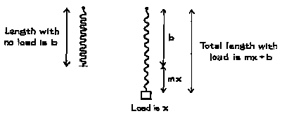
Let b be the length of the spring with no load. A weight of x kilograms is tied to the end of the spring. As illustrated in Figure 1, the spring stretches to a new length. According to Hooke's law, the amount of stretch is proportional to the weight x. So the new length of the spring is
y = mx + b.
In this equation, m and b are constants which depend on the spring. Their values are unknown and have to be estimated using experimental data.
Figure 4. Hooke's law: the stretch is proportional to the load.

Table 1 below shows the results of an experiment in which weights of various sizes were loaded on the end of a length of piano wire. 7 The first column shows the weight of the load. The second column shows the measured length. With 20 pounds of load, this "spring" only stretched about 0.2 inch (10 kg 22 lb, 0.5 cm @ 0.2 in). Piano wire is not very stretchy!
Table 1. Data on Hooke's law.
| Weight | Length |
| 0 kg | 439.00 cm |
| 2 | 439.12 |
| 4 | 439.21 |
| 6 | 439.31 |
| 8 | 439.40 |
| 10 | 439.50 |
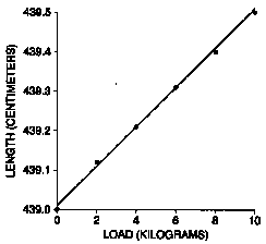
The correlation coefficient for these data is 0.999, very close to a perfect 1.0. So the points almost form a straight line (figure 2), just as Hooke's law predicts. The minor deviations from linearity are probably due to measurement error-neither the weights nor the lengths have been measured with perfect accuracy.
Figure 2. Scatter diagram for table 1.
Our goal is to estimate m and b in the equation of Hooke's law for the piano wire:
y = mx + b.
The graph of this equation is an ideal straight line, approximated by the scatter diagram in figure 2. If the points in figure 2 happened to fall exactly on some line, we would take that line as an approximation to the ideal line. Its slope would be an estimate for m, its intercept an estimate for b.
The trouble is that the points do not line up perfectly. Many different lines could be drawn across the scatter diagram, each having a slightly different slope and intercept. Which line should be used? Hooke's equation predicts length from weight. As discussed above, it is natural to choose m and b so as to minimize the r.m.s. error prediction error: this is the method of least squares. The line y = mx + b which does the job is the regression line. In other words, m in Hooke's law should be estimated as the slope of the regression line, and b as its intercept. These are called the least squares estimates, because they minimize root-mean-square error. Doing the arithmetic,
m = 0.05 cm per kg, and b = 439.01 cm.
The method of least squares estimates the length of the spring under no load to be 439.01 cm. And each kilogram of load causes the spring to stretch by an amount estimated as 0.05 cm. There is no need to hedge this statement, because it is based on a controlled experiment. The investigator puts the weights on, and the wire stretches. He takes the weights off, and the wire comes back to its original length. This process can be repeated as often as is desired.
Note that there is no question here about what is causing what: correlation is not causation, but in this experimental setting, the causation is clear and simple.
The method of least squares and the regression method involve the same mathematics; but the contexts may be different. In some fields, investigators talk about "least squares" when they are estimating parameters, like m and b in Hooke's law. In other fields, investigators talk about regression when they are studying the relationship between two variables, like income and education.
A technical point: The least squares estimate for the length of the spring under no load was 439.01 cm. This is a tiny bit longer than the measured length at no load (439.00 cm). A statistician would trust the least squares estimate over the measurement. Why? Because the least squares estimate takes advantage of all six measurements, not just one. Some of the measurement error is likely to cancel out. Of course, the six measurements are tied together by a good theory: Hooke's law. Without the theory, the least squares estimate wouldn't be worth much.
DOES THE REGRESSION MAKE SENSE?
A regression line can be put down on any scatter diagram. However, there are two questions to ask. First, was there a nonlinear association between the variables? If so, the regression line may be quite misleading. Even if the association looks linear, there is a second question: Did the regression make sense? The second question is harder. Answering it requires some understanding of the mechanism which produced the data. If this mechanism is not understood, fitting a line can be intellectually disastrous.
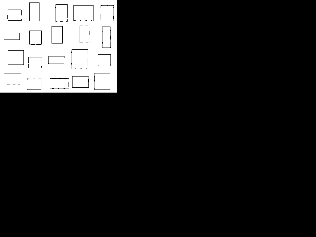
To make up an example, suppose an investigator does not know the formula for the area of a rectangle. Taking an empirical approach, she draws 20 typical rectangles, as shown in figure 3.
Figure 3. Twenty typical rectangles.
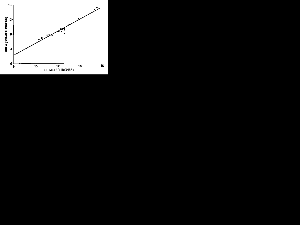
She thinks the area ought to depend on the perimeter (the distance you would travel if you walked around the outside of the rectangle). So for each rectangle she measures the area and the perimeter. A scatter diagram for the results is shown in figure 4 . The correlation coefficient turns out to be 0.98-almost as good as Hooke's law. The investigator concludes that she is really on to something. Her regression equation is
predicted area = (1.60 inches) · (perimeter) - 10.51 square inches.
(Area is measured in square inches and perimeter in inches.) The regression line is shown in figure 4.
Figure 4. Scatter diagram of area against perimeter, for the 20 rectangles in figure 3. The regression line is shown.
The arithmetic is all in order. But this investigator went at the problem so crudely that the equation is ridiculous. She should have looked at two other variables, length and width. These two variables determine both area and perimeter:
area = length · width,
perimeter = 2·(length + width).
Our straw-man investigator would never find this out by doing regressions.
Of course, this is just a made-up example. But many researchers do fit lines to scatter diagrams when they don't really know what's going on. This can make a lot of trouble. When thinking about a regression, ask yourself whether it is more like Hooke's law, or more like area and perimeter.
1. For the piano wire example discussed above, predict the length under the following loads, if possible: 3 kg, 7 kg, 50 kg.
2. The table below shows per capita disposable income and personal consumption expenditures, in 1982 dollars, yearly from 1960 to 1986.
(a) Find r and the regression equation for predicting consumption from income.
(b) Plot the residuals.
| Year | Income | Consumption |
| 1960 | 6,036 | 5,561 |
| 1961 | 6,113 | 5,579 |
| 1962 | 6,271 | 5,729 |
| 1963 | 6,378 | 5,855 |
| 1964 | 6,727 | 6,099 |
| 1965 | 7,027 | 6,362 |
| 1966 | 7,280 | 6,607 |
| 1967 | 7,513 | 6,730 |
| 1968 | 7,728 | 7,003 |
| 1969 | 7,891 | 7,185 |
| 1970 | 8,134 | 7,275 |
| 1971 | 8,322 | 7,409 |
| 1972 | 8,562 | 7,726 |
| 1973 | 9,042 | 7,972 |
| 1974 | 8,867 | 7,826 |
| 1975 | 8,944 | 7,926 |
| 1976 | 9,175 | 8,272 |
| 1977 | 9,381 | 8,551 |
| 1978 | 9,735 | 8,808 |
| 1979 | 9,829 | 8,904 |
| 1980 | 9,722 | 8,783 |
| 1981 | 9,769 | 8,794 |
| 1982 | 9,725 | 8,818 |
| 1983 | 9,930 | 9,139 |
| 1984 | 10,419 | 9,489 |
| 1985 | 10,622 | 9,830 |
| 1986 | 10,947 | 10,142 |
Note: Money variables are per capita, in 1982 dollars.
Source: Economic Report of the President, 1988, Table B-27.
predicted length = (0.05 cm per kg) x load + 439.01 cm
Substituting 3 kg and 7 kg for the load gives estimate lengths of 439.16 cm and 439.36 cm.
The method should not be used for a load of 50kg because 50kg is much bigger than anything
in Table 1 (and regression predictions are only valid for values of X that are within the
same general range as the values of X used to compute the regression equation). The wire
might snap.
(From Statistics, by Freedman, Pisani, Purves and Adhikari)