 CONNECTIONS 18(1):112-115.
Copyright 1995 INSNA
CONNECTIONS 18(1):112-115.
Copyright 1995 INSNA
Centrality measures are commonly described as indices of prestige, prominence, importance, and power -- the four Ps. However, this sort of interpretation seems inappropriate in the case of sexual networks. In this column, I consider the interpretation of centrality measures in sexual networks, and more generally in the context of any kind of network diffusion.
For simplicity, I will assume that the data consist of a discrete(1) symmetric social relation such as "has sex with", which we can represent as a binary adjacency matrix X in which aij = aji = 1 if actor i has sex with actor j and aij = aji = 0 otherwise. [In general, the same interpretations will hold for nonsymmetric data if we consider only incoming ties.]
Four measures of centrality are commonly used in network analysis: degree, closeness, betweenness, and eigenvector centrality. The first three were described in modern form by Freeman (1979) while the last was proposed by Bonacich (1972). Let us begin with degree.
Degree centrality may be defined as the number of ties that a given node has. More precisely, the degree of node i is given by:

In the case of the "has sex with" relation, the degree of an actor is simply the number of people she has sex with.
Suppose the probability of something occurring to an actor is a function of the number of exposures she has to it. For example, suppose the probability of adoption of an innovation is a function of the number of friends that a person witnesses adopting. Then we can interpret degree centrality in a friendship network as an index of the probability that they will adopt the innovation. All else being equal, then, we can describe degree centrality as measuring the risk (or opportunity) of receiving whatever is flowing through the network.
Eigenvector centrality is best understood as a variant of simple degree. Alexander (1963) had the idea that it wasn't just how many people a person knew that counted, but how many people the people that they knew knew. In the context of HIV transmission, we can see that all else being equal, a person A with one sex partner has a better chance of escaping the infection than a person B with many. But if that one sex partner that A has is having sex with most of the network, A's chances of getting infected are nearly as good as if she were having sex with all those others herself. This idea was anticipated by Katz (1953) and further developed by Hubbell (1965) and many others, finally culminating with Bonacich (1972) who defined centrality as the principal eigenvector of the adjacency matrix. An eigenvector of a symmetric square matrix A is any vector e which satisfies the equation

where is a constant (known as the eigenvalue) and ei gives the centrality of node i. The formula implies (recursively) that the centrality of a node is proportional to the sum of centralities of the nodes it is connected to. Hence, an actor that is connected to many actors who are themselves well-connected is assigned a high score by this measure, but an actor who is connected only to near isolates is not assigned a high score, even if she has high degree.
In the context of the risks or opportunities that a node faces to receive that-which-diffuses through the network, Bonacich's eigenvector centrality can be interpreted as a refined version of degree. Indeed, it can (generally) be computed by an iterative degree calculation, known as the accelerated power method (Hotelling 1936). The algorithm is as follows:
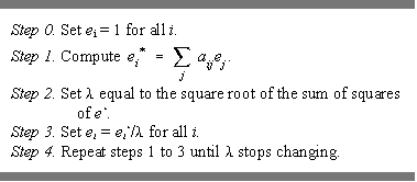
Note that after executing step 1 the first time, e* is equal to simple degree.
Closeness centrality may be defined as the total graph-theoretic distance of a given node from all other nodes. More precisely,
![]()
where dij is the number of links in the shortest path from actor i to actor j. Closeness is an inverse measure of centrality in that a larger value indicates a less central actor while a smaller value indicates a more central actor.
In the context of network diffusion, I interpret closeness as an index of the expected time-until-arrival at a given node of whatever is flowing through the network. To illustrate, suppose an infection enters a network at node p. Suppose also that it takes one unit of time to traverse a link. If we assume that the infection always travels along the shortest possible route(2), it will reach a given node q in dpq units of time, where dpq is the number of links in the shortest path from p to q. Now if the infection is equally likely to originate with any node in the network, then closeness centrality, ci is proportional to the expected number of time units until arrival of the infection at a given node.
Admittedly, few scientists view viruses as smart bombs programmed to find the shortest path to specific victims. In fact, the only way that a virus could take the shortest path to every node in any network is if, from any given node, it replicated and moved simultaneously to all adjacent nodes (something like news being relayed by ham radio broadcasts). However, my task here is not to find the best possible model of disease spread, but to interpret an existing model. Besides, in practice, the length of the shortest path between two nodes is highly correlated with the average length of all paths between the nodes. If the virus is equally likely to trace each possible path, closeness will not usually be far off the mark.
Betweenness centrality is more difficult to understand in this context. It may be defined loosely as the number of times that a node needs a given node to reach another node. More precisely (but not quite correctly), it is the number of shortest paths (between all pairs of nodes) that pass through a given node. It is exactly defined as

where gij is the number of shortest paths from node i to node j, and gikj is the number of shortest paths from i to j that pass through k. The purpose of the denominator is to provide a weighting system so that node k is given a full centrality point only when it lies along the only shortest path between i and j. If there is another equally short path that k is not on, k is given only a half a point, on the theory that the path that k is along has only a 0.5 chance of being chosen.
Betweenness indexes the extent to which a node's presence facilitates the flow of that-which-diffuses. If a node that is high on betweenness centrality is removed from the network, the speed and certainty of transmission from one arbitrary point to another are more damaged than if a node low on betweenness is removed.
Granovetter (1973) makes the same point about bridges and local bridges (which are ties rather than nodes). When a local bridge is removed, the nodes on either side of the bridge become reachable from each other only via very long paths. It is because Granovetter believes that only weak ties can be bridges that he makes his famous claim asserting the strength of weak ties. Actors with many weak ties are more important than others because removing those actors would do the most damage to transmission possibilities throughout the network.
To my mind, betweenness would clearly be a better way than counting weak ties to assess an actor's importance in the diffusion process -- if only that-which-diffuses did so in such a way as always travel along the best possible route.
Discussion.
While my main purpose has been simply to interpret existing centrality measures in the diffusion context, it is hard to ignore the fact that some of these existing measures (e.g., closeness, betweenness) do not seem up to the task. They work well if that-which-diffuses moves in all directions at once (thereby reaching every node via the shortest possible path), but not if it moves in just one direction at a time (e.g., the actors have sex with just one person at a time).
The obvious solution is to construct variants of closeness and betweenness that count all paths rather than just shortest paths. I am persuaded by Friedkin (1991) that off-the-shelf centrality measures are not as useful as measures custom-made for the particular empirical phenomenon of interest.
In constructing such measures, we might want to consider counting trails rather than strictly paths. A graph-theoretic path is a sequence of nodes in which no nodes are ever repeated. A trail is a sequence in which individual nodes may be repeated, but no adjacent pairs of nodes are repeated. For example, we might use trails to model the movement of a bit of gossip, because the same news may reach a given actor more than once from different source, yet it is unlikely (Alzheimer's aside!) that they would hear the story from the same person again.
1. In the mathematical sense, of course.
2. I know, I know. See next paragraph.
Alexander, C.N. 1963. "A method of processing sociometric data." Sociometry, 26:268-9.
Bonacich, P. 1972. "Factoring and weighting approaches to status scores and clique identification." Journal of Mathematical Sociology. 2:113-120.
Freeman, L.C. 1978. "Centrality in social networks: I. Conceptual clarification." Social Networks, 1:215-39.
Friedkin, N.E. 1991. "Theoretical foundations for centrality measures." American Journal of Sociology. 96:1478-504.
Granovetter, M.S. 1973. "The strength of weak ties." American Journal of Sociology. 78(6):1360-1380.
Hotelling, H. 1936. "Simplified calculation of principal components." Psychometrika. 1:27-35.
Hubbell, C.H. 1965. "An input-output approach to clique identification." Sociometry, 28:377-99.
Katz, L. 1953. "A new status index index derived from sociometric data analysis." Psychometrika, 18:39-43.