(Mr. Big, Sally),
(John, Billy),
(Sally, Peter),
(Sally, Mary),
(Mary, Falco)
The field of social network analysis uses three, highly related, areas of mathematics to represent networks: relations, graphs and matrices.
A binary relation R is a set of ordered pairs (x,y). Each element in an ordered pair is drawn from a (potentially different) set. The ordered pairs relate the two sets: together, they comprise a mapping, which is another name for a relation.
Functions, like y = 2x2 are relations. The equation notation is just short hand for enumerating all the possible pairs in the relation (e.g., (1,2), (3,18), (-2,8), etc.).
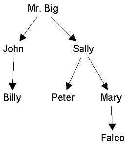
Social relations, which are at the heart of the network enterprise, correspond well to mathematical relations. To represent a social relation, such as "is the boss of", as a mathematical relation, we simply list all the ordered pairs:
| (Mr. Big, John), (Mr. Big, Sally), (John, Billy), (Sally, Peter), (Sally, Mary), (Mary, Falco) |
|
| Figure 1a. The "is the boss of" relation, represented as a binary relation. | Figure 1b. Same relation represented as a directed graph. |
A graph G(V,E) is a set of vertices (V) together with a set of edges (E). Some synonyms:
| Vertices | Edges | |
|---|---|---|
| Mathematics | node, point | line, arc, link |
| Sociology | actor, agent | tie |
There are several cross-cutting dimensions that distinguish among graphs.
| Directed vs Undirected: |
|
| Valued vs Non-Valued |
|
| Reflexive vs Non-Reflexive |
|
| Multi-graphs |
|
We represent graphs iconically as points and lines, such shown in Figure 1b. It is important to note that the location of points in space is arbitrary unless stated otherwise. This is because the only information in a graph is who is connected to whom. Hence, another, equally valid way to represent the graph in Figure 1 would be this:
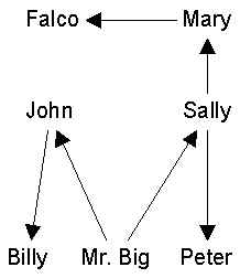
All representations in which the right people are connected to the right others are equally valid.
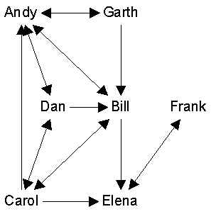
The degree of a node is the number of nodes it is adjacent to; or, equivalently, it is the number of edges that are incident upon it. A node with no degree (degree 0) is an isolate. A node with degree 1 is called a pendant. The graph in Figure 1 contains two pendants and no isolates.
In a digraph, the indegree of a node is the number of arcs coming in to a node from others, while the outdegree is the number of arcs from the node to all others. More technically, the indegree of a node u is |{(x,u): (x,u) E}|, where the vertical bar notation |S| gives the number of elements in set S. Similarly, the outdegree of u is given by |{(u,x): (u,x) E}|. A node with positive outdegree but no indegree is called a source. A node with positive indegree but no outdegree is called a sink.
A subgraph H of a graph G is a graph whose points and lines are also in G, so that V(H) V(G) and E(H) E(G). If we select a set of nodes S from a graph G, and then select all the lines that connect members of S, the resulting subgraph H is called an induced subgraph of G based on S. Two points are adjacent in H if and only if they are adjacent in G.
A walk is a sequence of adjacent points, together with the lines that connect them. In other words, a walk is an alternating sequence of points and lines, beginning and ending with a point, in which each line is incident on the points immediately preceding and following it. The points and lines in a walk need not be distinct. For example, in Figure 1, the sequence a-b-c-b-c-d is a walk. A path is a walk in which no node is visited more than once. The sequence a-b-c-d is a path. A cycle is like a path except that it begins and ends with the same node (e.g. c-d-e-c).
A set of walks that share no points is called vertex-disjoint. A set of walks that share no edges is called edge-disjoint. Obviously, vertex-disjoint paths are also edge-disjoint. If a pair of nodes are connected by three vertex-disjoint paths, this means that there are three, completely independent ways of getting from one point to the other. In Figure 1, there is only one edge-disjoint path from a to f, but two edge disjoint-paths from c to d.
The length of a walk is given by the number of lines it contains. A geodesic path is a shortest path between two points. There can be more than one geodesic path joining a given pair of points. The graph-theoretic distance or geodesic distance between two points is the length of a shortest path between them. In a diffusion process, one expects faster diffusion among nodes that are close together than among nodes that are far apart.
A graph is connected if there exists a path from every node to every other. A maximal connected subgraph is called a component. A maximal subgraph is a subgraph that satisfies some specified property (such as being connected) and to which no node can be added without violating the property. For example, in Figure 1, the subgraph induced by {a,b,c} is connected, but is not a component because it is not maximal: we could add node d and the subgraph induced would still be connected. The graph in Figure 1 has just one component, which is the whole graph.
A digraph that satisfies the connectedness definition given above (i.e. there exists a path from every node to every other) is called strongly connected. That is, for any pair of nodes a and b, there exists both a path from a to b and from b to a. A digraph is unilaterally connected if between every unordered pair of nodes there is at least one path that connects them. That is, for any pair of nodes a and b (and a b), there exists a path from either a to b or from b to a. A digraph whose underlying graph is connected is called weakly connected.
A maximal strongly connected subgraph is a strong component. A maximal weakly connected subgraph is a weak component. A maximal unilaterally connected subgraph is a unilateral component.
A cutpoint is a node whose removal would disconnect the graph. Alternatively, we could define a cutpoint as a node whose removal would increase the number of components of the graph. In the figure, nodes b, c, and e are cutpoints, while a, d, and f are not. A network that contains a cutpoint will break apart if the person who occupies the cutpoint leaves. A block is a subgraph which contains no cutpoints. A cutset is a set of points whose removal would disconnect a graph. A minimal cutset is a cutset that contains the minimum possible number of nodes that disconnect the graph. The size of a minimal cutset is called the vertex connectivity of the graph, and is denoted . The smaller the value of , the greater the vulnerability of the network to disconnection. We can also define a pairwise version of vertex connectivity, (u,v), which gives the minimum number of nodes that must be removed in order to disconnect vertex u from vertex v.
A bridge is a line whose removal disconnects the graph. An edge cutset is a set of lines whose removal disconnects the graph. A minimum weight cutset is an edge cutset which, for non-valued graphs, contains the fewest possible number of edges or, for valued-graphs, contains edges whose values add to the smallest possible value. The size of a minimum weight cutset is called the edge connectivity of the graph, and is denoted . As with point connectivity, we can also define a pairwise version of vertex connectivity, (u,v), which gives the minimum number of edges that must be removed in order to disconnect vertex u from vertex v.
Menger's theorem states that the minimum number of nodes that must be removed to disconnect node u from node v, (i.e. (u,v)) is equal to the maximum number of vertex-disjoint paths that join u and v. This also works for lines: the edge-connectivity (u,v) is equal to the maximum number of edge-disjoint paths that join u and v.
A good reference on graph theory is Frank Harary's 1969 book, Graph Theory, from Addison-Wesley.
We can record who is connected to whom on a given social relation via an adjacency matrix. The adjacency matrix is a square, 1-mode actor-by-actor matrix like this:
|
 |
||||||||||||||||||||||||||||||||||||||||||||||||||||||||||||||||
If the matrix as a whole is called X, then the contents of any given cell are denoted xij. For example, in the matrix above, xij = 1, because Andy likes Bill. Note that this matrix is not quite symmetric (xij not always equal to xji).
Anything we can represent as a graph, we can also represent as a matrix. For example, if it is a valued graph, then the matrix contains the values instead of 0s and 1s.
By convention, we normally record the data so that the row person "does it to" the column person. For example, if the relation is "gives advice to", then xij = 1 means that person i gives advice to person j, rather than the other way around. However, if the data not entered that way and we wish it to be so, we can simply transpose the matrix. The transpose of a matrix X is denoted X'. The transpose simply interchanges the rows with the columns.
Matrix Algebra
Matrices are basically tables. They are ways of storing numbers and other things. Typical matrix has rows and columns. Actually called a 2-way matrix because it has two dimensions. For example, you might have respondents-by-attitudes. Of course, you might collect the same data on the same people at 5 points in time. In that case, you either have 5 different 2-way matrices, or you could think of it as a 3-way matrix, that is respondent-by-attitude-by-time.
Notice that the rows and columns point to different class of entities. Rows are people, and columns are properties. Each different class of entities in a matrix is known as a mode. So this matrix is 2-way and 2-mode. Suppose we had a different matrix. Say we recorded the number of times that each of you spoke to each other of you. This would be a person-by-person matrix, which is 2-way 1-mode. If we tallied this up each month, we would have a person-by-person-by-month matrix, which would be 3-way, 2-mode.
A 1-way matrix is also called a vector. If it has rows but just one column, its a column vector. If it has columns but just one row its a row vector.
Typically, we refer to matrices using capital letters, like X. The number in a particular cell is identified via small letters and subscripts. Like x2,3. A generic cell in some row or some column is xij.
Although matrices are collections of numbers, they are also things in themselves. There are mathematical operations that you can define on them. For example, there is the transpose A’ where the rows become columns and vice versa.
For example, you can add them:
C = A+B
You can only perform these operations on matrices that are conformable. This means that they are of compatible sizes. Usually, that means they are the exact same size. For example, to add or subtract matrices, they must be the same size.
Multiplying matrices is a whole different thing. You write it this way: C=AB. First of all, you should know that matrix multiplication is not commutative. That is, it is not always true that AB=BA
Second, conformable in matrix multiplication means that the number of columns in the first matrix must equal the number of rows in the second.
Third, the product that results from a matrix multiplication has as many rows as the first matrix and as many columns as the second. so
A * B = C
3x2 * 2x4 = 3x4
Let A be
| 1 | 2 |
| 3 | 4 |
| 1 | 0 |
and B be
| 1 | 1 | 2 | 2 |
| 2 | 2 | 4 | 4 |
then C = AB is:
| 1*1+2*2 | 1*1+2*2 | 1*2+2*4 | 1*2+2*4 |
| 3*1+4*2 | 3*1+4*2 | 3*2+4*4 | 3*2+4*4 |
| 1*1+0*2 | 1*1+0*2 | 1*2+0*4 | 1*2+0*4 |
or
| 5 | 5 | 10 | 10 |
| 11 | 11 | 22 | 22 |
| 1 | 1 | 2 | 2 |
Note that we could not even try to multiply B*A, because they are not conformable.
What happens if we multiply A by matrix I which looks like this:
| 1 | 0 |
| 0 | 1 |
You get A back again! I is known as the identity matrix. It has 1s down the diagonal, and zeros elsewhere. Its almost always called I. When you multiply it by any matrix, you always get that matrix back again.
Now suppose you have an equation like
C = AB
and you have measured the values for C and for B, and would like to solve for the values of A. Can you do it?
Yes, but you can’t divide both sides by B. You can’t divide matrices at all. Just can’t do it. But you can multiply by the multiplicative inverse.
An inverse of an ordinary number is that thing you have to multiply the number by to get 1. The inverse of 2 is 0.5, because if you multiple 2*.5 you get 1.
In matrices, the inverse of B of is a matrix B-1 which when multiplied by B gets the identity matrix I, which is the matrix with all ones down the diagonal and zeros elsewhere.
If AB=BA=I, then A = B-1
So to find A in the equation C=AB, you postmultiply both sides by the inverse of B and get CB-1 = A.
This only works if B is square: same number of rows and columns.
Also, B must be non-singular. This means that none of the columns can be computed as a linear combination of any of the other columns. Same with the rows.
Postmultiplying matrix by a vector (Xb) is like computing weighted sum of rows. averaging across columns. if b is 1, then is just row sums. To get column sums, do btX or (Xtb)t
Eigenvectors and eigenvalues. The defining equation is Xv = kv, or kv = Xv, or v = k-1Xv or vi = k-1 xijvj
| Workshop Home | Steve Borgatti | Analytic Technologies | INSNA | Connections |