|
|
|
|
|
|
|
This exercise assumes you have access to the standard datasets that come with UCINET. These are automatically installed on your computer when you install UCINET. The default location is c:\program files\analytic technologies\ucinet 6\datafiles. For various reasons, you might prefer to copy this folder to a new location. For example, you might copy the Datafiles folder to your root directory, so that the new pathname would be c:\datafiles. This is a nice short path name! Whatever you decide to do, just remember where you put it and adjust the instructions below accordingly.
Setting Your Default Folder
It is *extremely* wise to start each UCINET session by setting the default folder to the folder containing the data you want to work on. Here’s how you do it.
Display some Data
In the menu, select Data|Display. At the “dataset:” prompt, press the ellipses (“..”) button to access file menu. Select a dataset called Campnet.
Note that what you see might be campnet.##h or campnet.##d. This is normal. The way UCINET stores data, the logical dataset CAMPNET is physically stored as two separate files, campnet.##h and campnet.##d, both of which are necessary. But you can refer to the dataset as campnet.##h or campnet.##d or just campnet: the program doesn’t care. It will be accessing both files no matter what.
Then press
“ok”. You should see something like this: -----------------------------------------------------------------------
Width of field: MIN # of decimals: MIN Rows to display: all Columns to display: all Row partition: Column partition: Input dataset: C:\Program Files\Analytic Technologies\Ucinet 6\datafiles\campnet
1 1 1 1 1 1 1 1 1 1 2 3 4 5 6 7 8 9 0 1 2 3 4 5 6 7 8 H B C P P J P A M B L D J H G S B R - - - - - - - - - - - - - - - - - - 1 HOLLY 0 0 0 1 1 0 0 0 0 0 0 1 0 0 0 0 0 0 2 BRAZEY 0 0 0 0 0 0 0 0 0 0 1 0 0 0 0 1 1 0 3 CAROL 0 0 0 1 1 0 1 0 0 0 0 0 0 0 0 0 0 0 4 PAM 0 0 0 0 0 1 1 1 0 0 0 0 0 0 0 0 0 0 5 PAT 1 0 1 0 0 1 0 0 0 0 0 0 0 0 0 0 0 0 6 JENNIE 0 0 0 1 1 0 0 1 0 0 0 0 0 0 0 0 0 0 7 PAULINE 0 0 1 1 1 0 0 0 0 0 0 0 0 0 0 0 0 0 8 ANN 0 0 0 1 0 1 1 0 0 0 0 0 0 0 0 0 0 0 9 MICHAEL 1 0 0 0 0 0 0 0 0 0 0 1 0 1 0 0 0 0 10 BILL 0 0 0 0 0 0 0 0 1 0 0 1 0 1 0 0 0 0 11 LEE 0 1 0 0 0 0 0 0 0 0 0 0 0 0 0 1 1 0 12 DON 1 0 0 0 0 0 0 0 1 0 0 0 0 1 0 0 0 0 13 JOHN 0 0 0 0 0 0 1 0 0 0 0 0 0 0 1 0 0 1 14 HARRY 1 0 0 0 0 0 0 0 1 0 0 1 0 0 0 0 0 0 15 GERY 0 0 0 0 0 0 0 0 1 0 0 0 0 0 0 1 0 1 16 STEVE 0 0 0 0 0 0 0 0 0 0 1 0 0 0 0 0 1 1 17 BERT 0 0 0 0 0 0 0 0 0 0 1 0 0 0 0 1 0 1 18 RUSS 0 0 0 0 0 0 0 0 0 0 0 0 0 0 1 1 1 0
---------------------------------------- Running time: 00:00:01 Output generated: 06 Jul 03 22:21:41 Copyright (c) 1999-2000 Analytic Technologies
Univariate Stats
Let’s run some basic statistics on the campnet dataset. Go to Tools|Univariate Stats. Where it says “Input Dataset:” type CAMPNET. Where it says “Which dimension to analyze” enter “Matrices” (use the down button to select matrix). Then press OK. The result should be:
UNIVARIATE STATISTICS --------------------------------------------------------------------------------
Dimension: MATRIX Diagonal valid? NO Input dataset: C:\Data\DataFiles\campnet
Descriptive Statistics
1 ------- 1 Mean 0.176 2 Std Dev 0.381 3 Sum 54.000 4 Variance 0.145 5 SSQ 54.000 6 MCSSQ 44.471 7 Euc Norm 7.348 8 Minimum 0.000 9 Maximum 1.000 10 N of Obs 306.000
Statistics saved as dataset C:\Data\DataFiles\campnet-uni
---------------------------------------- Running time: 00:00:01 Output generated: 11 Jul 04 23:31:57 Copyright (c) 1999-2004 Analytic Technologies
The mean of the matrix is .176. Since the matrix consists of 1s and 0s, you can interpret this mean as the number of 1s divided by the number of cells in the matrix (306). In other words, it is the proportion of cells that have value of 1.
Note that the stats you see on the screen are also saved as a file called campnet-uni. Most UCINET procedures produce two different kinds of outputs. One is the textual data that you see on the screen (reproduced in step 3 above). The other is a dataset (in this case called campnet-uni) saved on the hard disk.
Similarly, most procedures have two kinds of inputs: (a) a dataset (campnet), and (b) a set of choices of parameters, such as dimension = matrices.
More Stats
Suppose we re-run the Univariate Stats procedure choosing different parameters. In particular, where we said “matrices” last time let us change it to “rows” this time. The output should be:
UNIVARIATE STATISTICS --------------------------------------------------------------------------------
Dimension: ROWS Diagonal valid? NO Input dataset: C:\Data\DataFiles\campnet
Descriptive Statistics
1 2 3 4 5 6 7 8 9 10 Mean Std De Sum Varian SSQ MCSSQ Euc No Minimu Maximu N of O ------ ------ ------ ------ ------ ------ ------ ------ ------ ------ 1 HOLLY 0.176 0.381 3.000 0.145 3.000 2.471 1.732 0.000 1.000 17.000 2 BRAZEY 0.176 0.381 3.000 0.145 3.000 2.471 1.732 0.000 1.000 17.000 3 CAROL 0.176 0.381 3.000 0.145 3.000 2.471 1.732 0.000 1.000 17.000 4 PAM 0.176 0.381 3.000 0.145 3.000 2.471 1.732 0.000 1.000 17.000 5 PAT 0.176 0.381 3.000 0.145 3.000 2.471 1.732 0.000 1.000 17.000 6 JENNIE 0.176 0.381 3.000 0.145 3.000 2.471 1.732 0.000 1.000 17.000 7 PAULINE 0.176 0.381 3.000 0.145 3.000 2.471 1.732 0.000 1.000 17.000 8 ANN 0.176 0.381 3.000 0.145 3.000 2.471 1.732 0.000 1.000 17.000 9 MICHAEL 0.176 0.381 3.000 0.145 3.000 2.471 1.732 0.000 1.000 17.000 10 BILL 0.176 0.381 3.000 0.145 3.000 2.471 1.732 0.000 1.000 17.000 11 LEE 0.176 0.381 3.000 0.145 3.000 2.471 1.732 0.000 1.000 17.000 12 DON 0.176 0.381 3.000 0.145 3.000 2.471 1.732 0.000 1.000 17.000 13 JOHN 0.176 0.381 3.000 0.145 3.000 2.471 1.732 0.000 1.000 17.000 14 HARRY 0.176 0.381 3.000 0.145 3.000 2.471 1.732 0.000 1.000 17.000 15 GERY 0.176 0.381 3.000 0.145 3.000 2.471 1.732 0.000 1.000 17.000 16 STEVE 0.176 0.381 3.000 0.145 3.000 2.471 1.732 0.000 1.000 17.000 17 BERT 0.176 0.381 3.000 0.145 3.000 2.471 1.732 0.000 1.000 17.000 18 RUSS 0.176 0.381 3.000 0.145 3.000 2.471 1.732 0.000 1.000 17.000
Statistics saved as dataset C:\Data\DataFiles\campnet-uni
---------------------------------------- Running time: 00:00:01 Output generated: 12 Jul 04 08:20:04 Copyright (c) 1999-2004 Analytic Technologies
Each column of this matrix is a different statistic. For example, column 3 is the sum of each row in the Campnet matrix. In this case, each person has a sum of 3, indicating that they each have 3 outgoing ties.
Re-Displaying Data
Now run Data|Display on the dataset campnet-uni. The results should be the same as in the last step.
The Big D Button
Now we are going to display the CampAttr dataset (it might be called campattr2). But this time, use the shortcut icon on the toolbar that is labeled with a big “D”. The output should look like this:
DISPLAY --------------------------------------------------------------------------------
Width of field: MIN # of decimals: MIN Rows to display: all Columns to display: all Row partition: Column partition: Input dataset: C:\Program Files\Ucinet 6\workshop\campattr
1 2 3 G R C - - - 1 HOLLY 1 1 1 2 BRAZEY 1 1 1 3 CAROL 1 1 1 4 PAM 1 1 1 5 PAT 1 1 1 6 JENNIE 1 1 1 7 PAULINE 1 1 1 8 ANN 1 1 1 9 MICHAEL 2 1 2 10 BILL 2 1 2 11 LEE 2 1 2 12 DON 2 1 2 13 JOHN 2 1 2 14 HARRY 2 1 2 15 GERY 2 2 3 16 STEVE 2 2 3 17 BERT 2 2 3 18 RUSS 2 2 3
Bank Wiring Room Dataset
You start by going to Help|Help Topics and then clicking on “Standard Datasets”. Then click on “ROETHLISBERGER & DICKSON BANK WIRING ROOM” and read the description of the data.
Now display (again use shortcut key combination Ctrl-D) the Wiring dataset. Should look like this:
DISPLAY --------------------------------------------------------------------------------
Width of field: MIN # of decimals: MIN Rows to display: all Columns to display: all Row partition: Column partition: Input dataset: C:\Program Files\Ucinet 6\datafiles\wiring
Matrix #1: RDGAM
1 1 1 1 1 1 2 3 4 5 6 7 8 9 0 1 2 3 4 I I W W W W W W W W W S S S - - - - - - - - - - - - - - 1 I1 0 0 1 1 1 1 0 0 0 0 0 0 0 0 2 I3 0 0 0 0 0 0 0 0 0 0 0 0 0 0 3 W1 1 0 0 1 1 1 1 0 0 0 0 1 0 0 4 W2 1 0 1 0 1 1 0 0 0 0 0 1 0 0 5 W3 1 0 1 1 0 1 1 0 0 0 0 1 0 0 6 W4 1 0 1 1 1 0 1 0 0 0 0 1 0 0 7 W5 0 0 1 0 1 1 0 0 1 0 0 1 0 0 8 W6 0 0 0 0 0 0 0 0 1 1 1 0 0 0 9 W7 0 0 0 0 0 0 1 1 0 1 1 0 0 1 10 W8 0 0 0 0 0 0 0 1 1 0 1 0 0 1 11 W9 0 0 0 0 0 0 0 1 1 1 0 0 0 1 12 S1 0 0 1 1 1 1 1 0 0 0 0 0 0 0 13 S2 0 0 0 0 0 0 0 0 0 0 0 0 0 0 14 S4 0 0 0 0 0 0 0 0 1 1 1 0 0 0
------------------------------------------
Matrix #2: RDCON
1 1 1 1 1 1 2 3 4 5 6 7 8 9 0 1 2 3 4 I I W W W W W W W W W S S S - - - - - - - - - - - - - - 1 I1 0 0 0 0 0 0 0 0 0 0 0 0 0 0 2 I3 0 0 0 0 0 0 0 0 0 0 0 0 0 0 3 W1 0 0 0 0 0 0 0 0 0 0 0 0 0 0 4 W2 0 0 0 0 0 0 0 0 0 0 0 0 0 0 5 W3 0 0 0 0 0 0 0 0 0 0 0 0 0 0 6 W4 0 0 0 0 0 0 1 1 1 0 1 0 0 0 7 W5 0 0 0 0 0 1 0 1 0 0 0 1 0 0 8 W6 0 0 0 0 0 1 1 0 1 1 1 1 0 1 9 W7 0 0 0 0 0 1 0 1 0 1 1 0 0 1 10 W8 0 0 0 0 0 0 0 1 1 0 1 1 0 1 11 W9 0 0 0 0 0 1 0 1 1 1 0 1 0 0 12 S1 0 0 0 0 0 0 1 1 0 1 1 0 0 1 13 S2 0 0 0 0 0 0 0 0 0 0 0 0 0 0 14 S4 0 0 0 0 0 0 0 1 1 1 0 1 0 0
------------------------------------------ .. ..
(several more matrices)
Note that the Wiring dataset contains multiple networks, each represented as a binary matrix.
Now let’s run univariate statistics on the Wiring dataset, choosing “Matrices” as the dimension to analyze:
UNIVARIATE STATISTICS --------------------------------------------------------------------------------
Dimension: MATRIX Diagonal valid? NO Input dataset: C:\Data\DataFiles\wiring
Descriptive Statistics
1 ------- 1 Mean 0.308 2 Std Dev 0.462 3 Sum 56.000 4 Variance 0.213 5 SSQ 56.000 6 MCSSQ 38.769 7 Euc Norm 7.483 8 Minimum 0.000 9 Maximum 1.000 10 N of Obs 182.000
Descriptive Statistics
1 ------- 1 Mean 0.209 2 Std Dev 0.406 3 Sum 38.000 4 Variance 0.165 5 SSQ 38.000 6 MCSSQ 30.066 7 Euc Norm 6.164 8 Minimum 0.000 9 Maximum 1.000 10 N of Obs 182.000
Descriptive Statistics
1 ------- 1 Mean 0.143 2 Std Dev 0.350 3 Sum 26.000 4 Variance 0.122 5 SSQ 26.000 6 MCSSQ 22.286 7 Euc Norm 5.099 8 Minimum 0.000 9 Maximum 1.000 10 N of Obs 182.000
Descriptive Statistics
1 ------- 1 Mean 0.209 2 Std Dev 0.406 3 Sum 38.000 4 Variance 0.165 5 SSQ 38.000 6 MCSSQ 30.066 7 Euc Norm 6.164 8 Minimum 0.000 9 Maximum 1.000 10 N of Obs 182.000
Descriptive Statistics
1 ------- 1 Mean 0.132 2 Std Dev 0.338 3 Sum 24.000 4 Variance 0.114 5 SSQ 24.000 6 MCSSQ 20.835 7 Euc Norm 4.899 8 Minimum 0.000 9 Maximum 1.000 10 N of Obs 182.000
Descriptive Statistics
1 ------- 1 Mean 0.269 2 Std Dev 1.827 3 Sum 49.000 4 Variance 3.340 5 SSQ 621.000 6 MCSSQ 607.808 7 Euc Norm 24.920 8 Minimum 0.000 9 Maximum 20.000 10 N of Obs 182.000
Statistics saved as dataset C:\Data\DataFiles\wiring-uni
---------------------------------------- Running time: 00:00:01 Output generated: 12 Jul 04 08:27:44 Copyright (c) 1999-2004 Analytic Technologies
The result is a set of statistics for each matrix contained in the Wiring dataset.
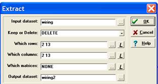
Extracting Data
Let’s eliminate the isolates from a network – i.e., nodes that have no ties. Go to Data|Extract. Fill out the prompts as follows:
And obtain the following results:
EXTRACT --------------------------------------------------------------------------------
Operation: DELETE Rows: 2 13 Columns: 2 13 Relations: NONE Input dataset: C:\Program Files\Ucinet 6\datafiles\wiring Output dataset: wiring2
Matrix 1: RDGAM
1 1 1 1 1 3 4 5 6 7 8 9 0 1 2 4 I W W W W W W W W W S S - - - - - - - - - - - - 1 I1 0 1 1 1 1 0 0 0 0 0 0 0 3 W1 1 0 1 1 1 1 0 0 0 0 1 0 4 W2 1 1 0 1 1 0 0 0 0 0 1 0 5 W3 1 1 1 0 1 1 0 0 0 0 1 0 6 W4 1 1 1 1 0 1 0 0 0 0 1 0 7 W5 0 1 0 1 1 0 0 1 0 0 1 0 8 W6 0 0 0 0 0 0 0 1 1 1 0 0 9 W7 0 0 0 0 0 1 1 0 1 1 0 1 10 W8 0 0 0 0 0 0 1 1 0 1 0 1 11 W9 0 0 0 0 0 0 1 1 1 0 0 1 12 S1 0 1 1 1 1 1 0 0 0 0 0 0 14 S4 0 0 0 0 0 0 0 1 1 1 0 0
…
What you have just done is to create a new dataset called Wiring2 that is just like the original except that it is missing the two nodes (I3 and S2).
UCINET Spreadsheet
Go to Data|Spreadsheet and open the Wiring2 dataset that you just created. Verify that I3 and S2 are gone.
Press the
|
|